Example 1
Ziptool can be used with downloaded CSV files of ACS data, but it works best with ipumspy, a Python package that uses your IPUMS API key to pull data directly. The example below details a sample use case of ziptool for basic demographic research using ipumspy and both implementations of data_by_zip.
In this example, we want to explore various demographic traits of five coastal New England towns throughout the region: Jamestown, RI (02835); Kennebunkport, ME (04046); New Bedford, MA (02740); Stonington, CT (06355); and Westerly, RI (02804). We are particularly interested in household income and ancestry.
Setup
First, import pandas, numpy, and some other important dependencies.
import pandas as pd
import numpy as np
from pathlib import Path
We give two options for pulling data. Using ipumspy is recommended as it is much easier to use, but importing CSVs is fully supported as well.
Option 1: Manually Pulling Data
Go to https://usa.ipums.org/usa/ and create a free account.
Click the “Select Data” tab.
Click “Select Samples” to select the year of ACS data you are interested in
(ziptool only supports one year at a time).
4. Under the “Select Harmonized Variables” dropdown, choose the variables you would like. Be sure to add “PUMA” and “STATEFIP” under the Household -> Geographic tab 5. Hit “View Cart” then select “Create Data Extract.” Select .csv as the data format and rectangular under structure. 6. Hit submit extract and wait until it is finished so you can download!
Once you have the data downloaded, simply pass the path to the CSV as an argument in data_by_zip. Ziptool will handle the import for you.
The rest of the tutorial will use the ipumspy option because of its ability to import and parse the associated codebook, which we need in this example.
Option 2: Pulling Data with ipumspy
Import ipumspy and the modules we need explicitly.
import ipumspy
from ipumspy import IpumsApiClient, UsaExtract, readers, ddi
Then, using the API key, we request the variable we are interested in (‘HHINCOME’ and ‘ANCESTR1’) along with ‘PUMA’ and ‘STATEFIP’, both of which are required variables for usage with ziptool. We also would like to get data from the 2019 ACS, which is labeled in ipums as ‘us2019a’. The request is then submitted and downloaded (note that this can take quite a while depending on how many variables you request.)
IPUMS_API_KEY = your_api_key
DOWNLOAD_DIR = Path(your_download_dir)

ipums = IpumsApiClient(IPUMS_API_KEY)

extract = UsaExtract(
    ["us2019a"],
    ["STATEFIP","PUMA","HHINCOME","ANCESTR1"],
)
ipums.submit_extract(extract)
ipums.wait_for_extract(extract)
ipums.download_extract(extract, download_dir=DOWNLOAD_DIR)
Continuous Variables
Now all the data needed for analysis is downloaded, and we can read it in as a pd.DataFrame along with the codebook that contains the information associated with each variable so that we can properly conduct our analysis.
ddi_file = list(DOWNLOAD_DIR.glob("*.xml"))[0]
ddi = ipumspy.readers.read_ipums_ddi(ddi_file)

ipums_df = ipumspy.readers.read_microdata(ddi,
            DOWNLOAD_DIR / ddi.file_description.filename)
In this example, we want to analyze two different traits for these communities: mean household income and reported ancestry. The former is a numerical ratio variable whereas the latter is categorical. That means that we can take advantage of ziptool’s built-in analysis functions for HHINCOME but will read in the raw data for the categorical data of ‘ANCESTR1’. We import the relevant modules of ziptool, data_by_zip (which will calculate the ZIP-level data) and convert_to_df (which will convert the returned data into a pd.DataFrame for easier analysis). Because we only want to analyze HHINCOME using summary statisticcs, we pass only ‘HHINCOME’ as a variable of interest. The null value comes from the codebook, as does the type (household vs. individual variable).
from ziptool.query_by_zip import data_by_zip
from ziptool.utils import convert_to_df

income_data = data_by_zip(['02835','04046','02740','06355','02804'], ipums_df,
    {"HHINCOME": {"null": 9999999, "type":'household'}})
We now have a pd.DataFrame, income_data, that contains all of our data! We can easily generate a bar plot to visualize differences by income as an example of the easy analysis that we can now perform.
import matplotlib.pyplot as plt
ylgnbu = ['#7fcdbb', '#41b6c4', '#225ea8',
          '#0c2c84', '#f29c33', '#666462']
#defining our colorscale

plt.bar(income_df.index, income_df['HHINCOME_mean'], color = ylgnbu[3])
plt.title('Average Household Income')
plt.show()

Categorical Variables
Categorical variables like ANCESTR1 are not usefully summarized by summary statistics, so in this case, we can read in the raw data and perform our own analysis. We do this by simply not specifying any variables:
raw_dfs = data_by_zip(['02835','04046','02740','06355','02804'], ipums_df)
We are particularly interested in four ancestral groups that often formed much of the populations of some coastal New England towns in the late 1800s : people of Portuguese, Irish, Italian, and English ancestry. However, countries are encoded as numbers in ‘ANCESTR1’ fron the ACS, so we must access the codebook to pull out the codes corresponding to the ancestries we are interested in.
ancestry_info = ddi.get_variable_info('ANCESTR1')
ancestry_codes = ancestry_info.codes
top_codes = [ancestry_codes['Portuguese'],
             ancestry_codes['Irish, various subheads,'],
             ancestry_codes['Italian'],
             ancestry_codes['English']]
We can now plot a pie chart of each ZIP code’s ancestry demographics:
fig, ax = plt.subplots(2,3)

for i,zip in enumerate(['02835','04046','02740','06355','02804']):
    row = int(np.floor(i/3))
    column = int(i % 3)
    data = raw_dfs[zip]
    ancestry_data= data.groupby('ANCESTR1').sum()['PERWT']
    other = pd.Series([ancestry_data.loc[~ancestry_data.index.isin(top_codes + [ancestry_codes['Not Reported']])].sum()],index=[0])
    to_plot = ancestry_data[top_codes].append(other)
    ax[row,column].pie(to_plot, colors = ylgnbu)
    ax[row,column].set_title(zip)

ax[1,2].axis('off')
fig.legend(['Portuguese','Irish','Italian','English','Other'], loc = 4)
plt.show()
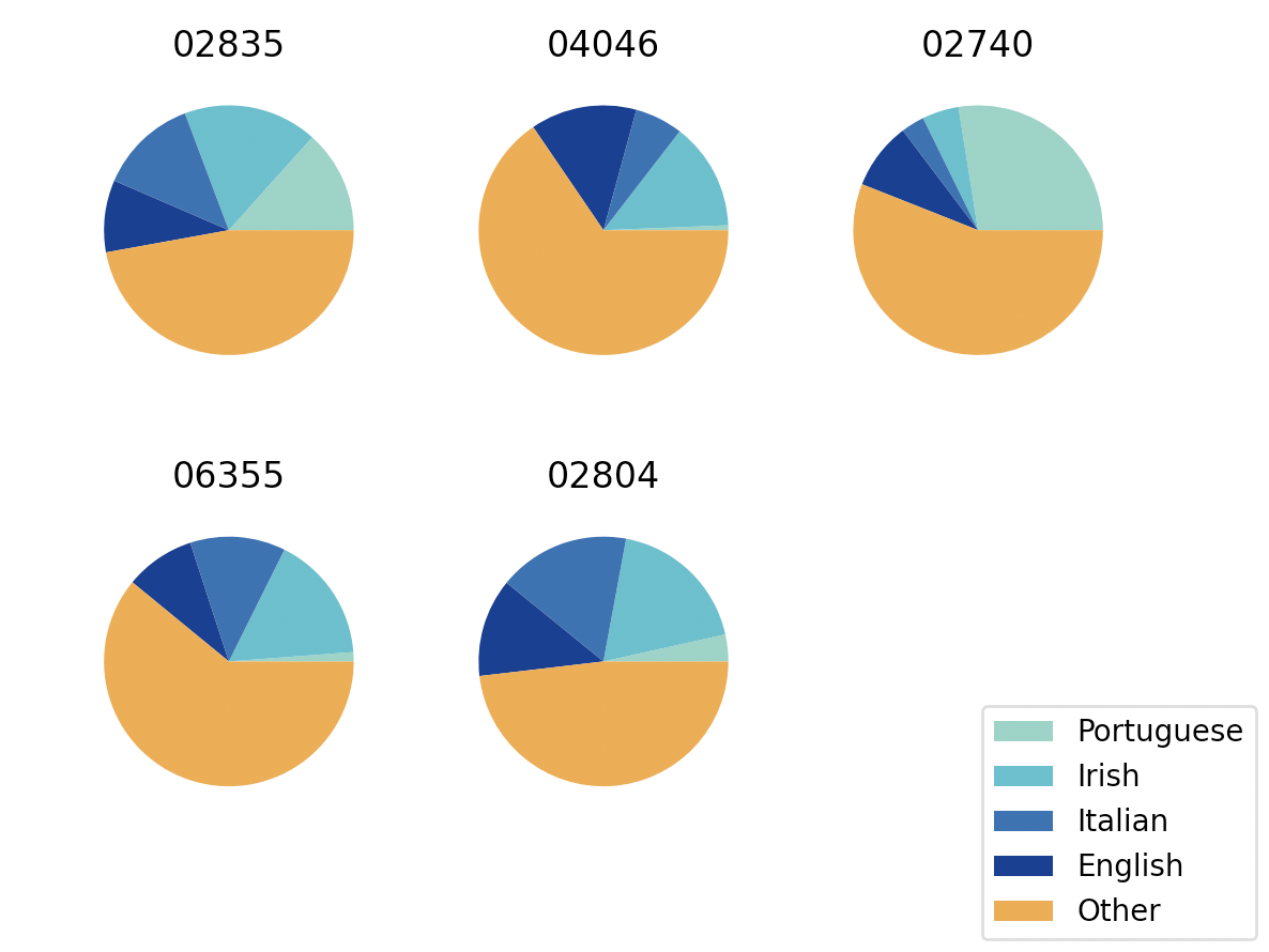
And just like that, we have analyzed our categorical variable! You can manipulate, analyze, and visualize display data like you normally would with the ZIP-level data in a standard pd.DataFrame!