Example 2

Here, we are interested in comparing the correlations between different household variables for different variables. We will use ipumspy and ziptool to easily extract this data and generate correlation matrices.

Setup

First, import pandas, ziptool, ipumspy and some plotting mechanisms.

import sys
from configuration import *
import pandas as pd
from pathlib import Path
import matplotlib.pyplot as plt
import seaborn as sns
import ipumspy
from ipumspy import IpumsApiClient, UsaExtract, readers, ddi

from ziptool.query_by_zip import data_by_zip

First, we pull our data using ipumspy.

Fetching Data

Using our API key, we request the variables we are interested in (a selection of household dwelling and economic indicators) along with ‘PUMA’ and ‘STATEFIP’, both of which are required variables for usage with ziptool. We also would like to get data from the 2019 ACS, which is labeled in ipums as ‘us2019a’. The request is then submitted and downloaded (note that this can take quite a while).

IPUMS_API_KEY = your_api_key
DOWNLOAD_DIR = Path(your_download_dir)

ipums = IpumsApiClient(IPUMS_API_KEY)

extract = UsaExtract(
    ["us2019a"],
    ["STATEFIP","PUMA","HHINCOME","ROOMS","BEDROOMS", \
     "CIHISPEED","FUELHEAT","VEHICLES","VALUEH"],
)
ipums.submit_extract(extract)
ipums.wait_for_extract(extract)
ipums.download_extract(extract, download_dir=DOWNLOAD_DIR)

Analyzing The Data

Now all the data needed for analysis is downloaded, and we can read it in as a pd.DataFrame along with the codebook that contains the information associated with each variable so that we can properly conduct our analysis.

ddi_file = list(DOWNLOAD_DIR.glob("*.xml"))[0]
ddi = ipumspy.readers.read_ipums_ddi(ddi_file)

ipums_df = ipumspy.readers.read_microdata(ddi,
            DOWNLOAD_DIR / ddi.file_description.filename)

First, we define the null values of each of our variables (obtained from the IPUMS online codebook).

HHINCOME_null = 9999999
BEDROOMS_null = 0
ROOMS_null = 0
CHISPEED_null = 0
FUELHEAT_null = 0
VEHICLES_null = 0
VALUEH_null = 9999999

Then, we define a function called compare_variables which takes in a list of zip codes and computes / plots the cross-correlation matrix between each variable of interest. We first use ziptool’s data_by_zip function to return the raw dataframes for each ZIP code (we do not want any intermediate analysis or summary statistics) and remove the null values for each zip code; we then pre-process the CIHISPEED variable to transform it from a categorical variable to a binary variable (i.e. does a household have broadband access, not what kind). Then, we generate a heatmap and plot!

def compare_variables(zips):

    fig, axes = plt.subplots(1,len(zips), figsize = (12,4))

    df = data_by_zip(zips, ipums_df)

    for index, (zip, value) in enumerate(df.items()):

        mask = [value["BEDROOMS"] > BEDROOMS_null] and [value["ROOMS"] > ROOMS_null] and \
        [value["CIHISPEED"] > CHISPEED_null] and [value["FUELHEAT"] > FUELHEAT_null] and \
        [value["VEHICLES"] > VEHICLES_null] and [value["VALUEH"] != VALUEH_null] and \
        [value["HHINCOME"] != HHINCOME_null ]

        filtered = value[mask[0]]

        oneperson = filtered[filtered['PERNUM'] == 1]
        oneperson['CIHISPEED'] = oneperson['CIHISPEED'].replace(20,0)
        oneperson['CIHISPEED'] = oneperson['CIHISPEED'].replace([10,11,12,13,14,15,16,17],1)

        sns.heatmap(oneperson[["HHINCOME","ROOMS","BEDROOMS","CIHISPEED","VEHICLES","VALUEH"]].multiply(oneperson['HHWT'],axis = 'index').corr(), cmap = 'YlGnBu', vmin = 0, vmax = 1, ax = axes[index])
        axes[index].set_title(zip)

    plt.tight_layout()

Now that the function is defined, we can simply call it for whichever variables we are interested in.

compare_variables(['02835','10001','79901'])

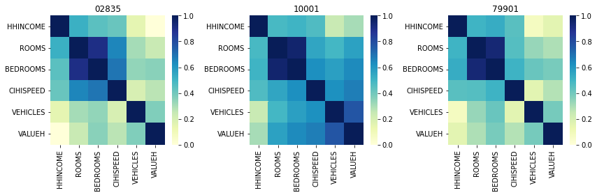
Boom! We’ve used ziptool to extract ZIP-level data which we can use to perform advanced geographical analyses for any variables we would like.